Defining Confidence Levels for UKB Round 2 LDSR Analyses
Results from the Neale Lab
Last updated 2022-10-11
Overview
Elsewhere we’ve described how we selected a “primary” \(h^2_g\) result for each of the unique phenotypes in the UKB GWAS. These phenotypes range widely in terms of sample size and polygenicity, among other factors. These features can affect our confidence in the stability of the LD Score Regression results. For example we previously noted concerns about bias at low effective sample sizes.
We document here out evaluation of confidence in each of the LDSR \(h^2_g\) results. This is separate from our evaulation of statistical significance for these results. Here we look at:
- What is the minimum sample size necessary to have statistical power for LDSR \(h^2_g\) estimation?
- Are there signs of bias in \(h^2_g\) estimates as a function of sample size?
- Are there phenotypes with unexpectedly large sampling variation for their \(h^2_g\) estimate?
- Are there phenotyping features to be aware of in assessing our confidence in interpreting the results?
We conclude with a summary of our current confidence classifications.
Minimum sample size
After we’ve defined a “primary” \(h^2_g\) result for each of the 4178 unique phenotypes in the Round 2 GWAS, we know that the sample size (or effective sample size) for many of these phenotypes is quite low. For example, case counts are quite small for most ICD codes and job codes. To avoid unnecessary multiple testing for the significance of the \(h^2_g\) results we therefore aim to identify the minimum (effective) sample size required to provide sufficient power to make LDSR analysis viable. [NB: We focus first on a bare minimum in terms of power, we’ll return to the question of bias later.]
Goal: determine the minimum (effective) sample size where we’d expect to have some useful level of power to detect a reasonable \(h^2_g\).
Question 1: What’s the relationship between sample size and precision for LDSR?
To evaluate the effective sample size required to have power in LDSR analyses, we consider the relationship between \(N_{eff}\) and the observed standard error (SE) for the LDSR \(h^2_g\) estimate for the 4178 Round 2 phenotypes.
Takeaway: There’s a clear inverse relationship between \(N_{eff}\) and the SE of the \(h^2_g\) estimate. The SE is also very large (e.g. wider than the 0-1 range for \(h^2\)) at small effective sample sizes.
For both visualization and modelling, it’s useful to look at this relationship in terms of the inverse variance (\(1/SE^2\)):
Takeaway: There’s a nearly linear relationship between \(N_{eff}\) and \(1/SE^2\). This relationship is highly heteroskedastic, with much greater variability in the inverse variance when \(N_{eff}\) is large.
We can model this observed relationship in order to establish the “expected” inverse variance as a function of \(N_{eff}\). Given the observed heteroskedasticity, and that our primary interest is in the error variance at small sample sizes, we consider a weighted regression with weights inversely proportional to sample size. Based on the plot above we also allow for quadratic curvature in the relationship with \(N_{eff}\), and also compare regression to a loess fit.
Of these, the loess fit appears to better fit the overall trend of the data, especially when focusing on smaller sample sizes (as is visible when zooming the above plot). Note the smaller sample sizes are the range relevant to the current question of the minimum viable sample size for ldsc.
We adopt the loess model (green) for predicting SEs from sample size for the rest of this section.
Question 2: Power as a function of expected SE
Given the above model for expected SEs as a function of sample size, and assuming the SEs are well calibrated, we can then turn these modelled SEs into a power analysis.
Specifically, we ask for a given true SNP heritability, sample size and p-value threshold what the probability is of the estimated \(h^2_g\) divided by its SE exceeding to corresponding critical value for the Z statistic, assuming the sampling variation of the estimated estimated \(h^2_g\) and it’s estimated SE both match the expected SE based on sample size given by the above model. We focus on here power at \(p < .05\) without any multiple testing correction in the interest of providing results relevant to hypotheses that include look-ups of \(h^2_g\) for a single phenotype (as opposed to scans across all available UKB phenotypes). We’ll return to the question of which results we’d consider significant in the context of looking at all 4178 phenotypes later.
Note that this is a bit more empirical than a formal power analysis. We’re relying on the average observed SE reported for the ldsc \(h^2_g\) estimates rather than some theoretical expectation for the SE. There’s also likely a relationship between the SE and the true \(h^2_g\) (and corresponding genetic architecture), as evidenced by the previous plots of precision vs. sample size colored by \(h^2_g\) estimate, that we do not account for in this power estimate. Nevertheless, we use this modelled estimate of power as a useful rough benchmark for evaluating what range of sample sizes to include in this \(h^2_g\) analysis.
Question 3: What \(h^2_g\) is worth detecting?
Now that we have rough estimates of power as a function of \(h^2_g\) and sample size, the question is what \(h^2_g\) is relevant to have power to detect.
If we look at the UKB phenotypes with the larges sample sizes (i.e. \(N_{eff}\)>300k, where there’s no worry about power) we find that the vast majority of phenotypes have \(h^2_g\) estimates \(\leq 0.3\), with a somewhat bimodal distribution (overall mean=0.118, median=0.078).
From the observed \(h^2_g\) distribution, is appears the phenotypes with larger estimated SNP heritability tend to have estimates around \(h^2_g=0.2\) or slightly larger. We can then orient our decisions on sample size around having power to detect \(h^2_g \geq 0.2\).
Conclusion
From the above estimated power analysis, based on a loess fit of the observed SE of \(h^2_g\) estimates as a function of effective N, we estimate needing \(N_{eff}\)=4565.48 to have at least 80% power to detect \(h^2_g \geq 0.2\) at nominal significance (\(p < .05\)). We take 80% power as a standard goal for having a “well-powered” analysis, and focus on \(h^2_g \geq 0.2\) and \(p < .05\) for the reasons described above.
For the sake of having a round number, and choosing to err slightly towards being inclusive in the analysis, we take this fitted value and round down to \(N_{eff}=4500\). We exclude 2298 phenotypes with \(N_{eff} \leq 4500\) from further consideration in the LDSR \(h^2_g\) analysis based on this threshold, leaving 1880 phenotypes.
[NB: We’re lenient here largely because we know much more stringent criteria on \(N_{eff}\) will be applied below in defining “low confidence” results.]
Potential small sample biases
The above set of conditions identifies 1880 phenotypes that avoid redundancy for encoding and sex-specific results and reach a minimum effective sample size (\(N_{eff}\)) necessary for LDSR analysis to be viable in terms of power. These thresholds may be considered a bare minimum. We now consider instances among these 1880 phenotypes where we may still be pessimistic about the accuracy of the LDSR results.
In the first round of UKB GWAS from the Neale lab, we highlighted possible biases in the LDSR \(h^2_g\) estimate at low \(N_{eff}\). In particular, we observed signs of attenuated \(h^2_g\) estimates for phenotypes with \(N_{eff} < 10,000\). We reassess that trend here.
Note: Plot restricted to 1880 phenotypes passing \(N_{eff}\) threshold. Zoom out to see \(h^2_g\) outliers.
Takeway: Some mild attenuation in \(h^2_g\) is seen below \(N_{eff} = 100,000\), but it’s as not as severe nor as sharply limited to \(N_{eff} < 10,000\) as observed in round 1.
Question 1: results changed as a function of mix of questions?
One possible hypothesis is that the change in the shape of attenuation reflects the changing mix of phenotypes in the Round 2 GWAS release. In particular, there’s a large number of additional diet items with \(N_{eff} \approx 50,000\) and mental health items at \(N_{eff} \approx 120,000\). It’s possible these subsets of items are influencing the shape of the attentuation curve by confounding true \(h^2_g\) with \(N_{eff}\). If we restrict to variables observed in nearly all samples:
Takeaway: the milder attentuation of \(h^2_g\) as a function of \(N_{eff}\) is still observed when restricting to 963 phenotypes with \(N > 300,000\). Similar trends are observed for subsetting on other dimensions (not shown).
Conclusion: The mix of phenotypes doesn’t appear to explain the weaker attentuation effect.
Question 2: Attentuation evident in downsampling?
Instead of looking across phenotypes, we can also consider the impact of sample size on \(h^2_g\) estimates within a phenotype. We evaluate this by looking at how the LDSR estimates change when subsetting individuals from UKB for phenotypes with high \(N\)s and strong \(h^2_g\) estimates.
Specifically, for a given downsampling experiment we split UKB individuals into 300 chunks, perform a GWAS within each chunk (controlling for the standard GWAS covariates), and then meta-analyze increasing numbers of chunks. We then run LDSR for each of these meta-analyses to assess how the \(h^2_g\) estimates change with growing meta-analyses.
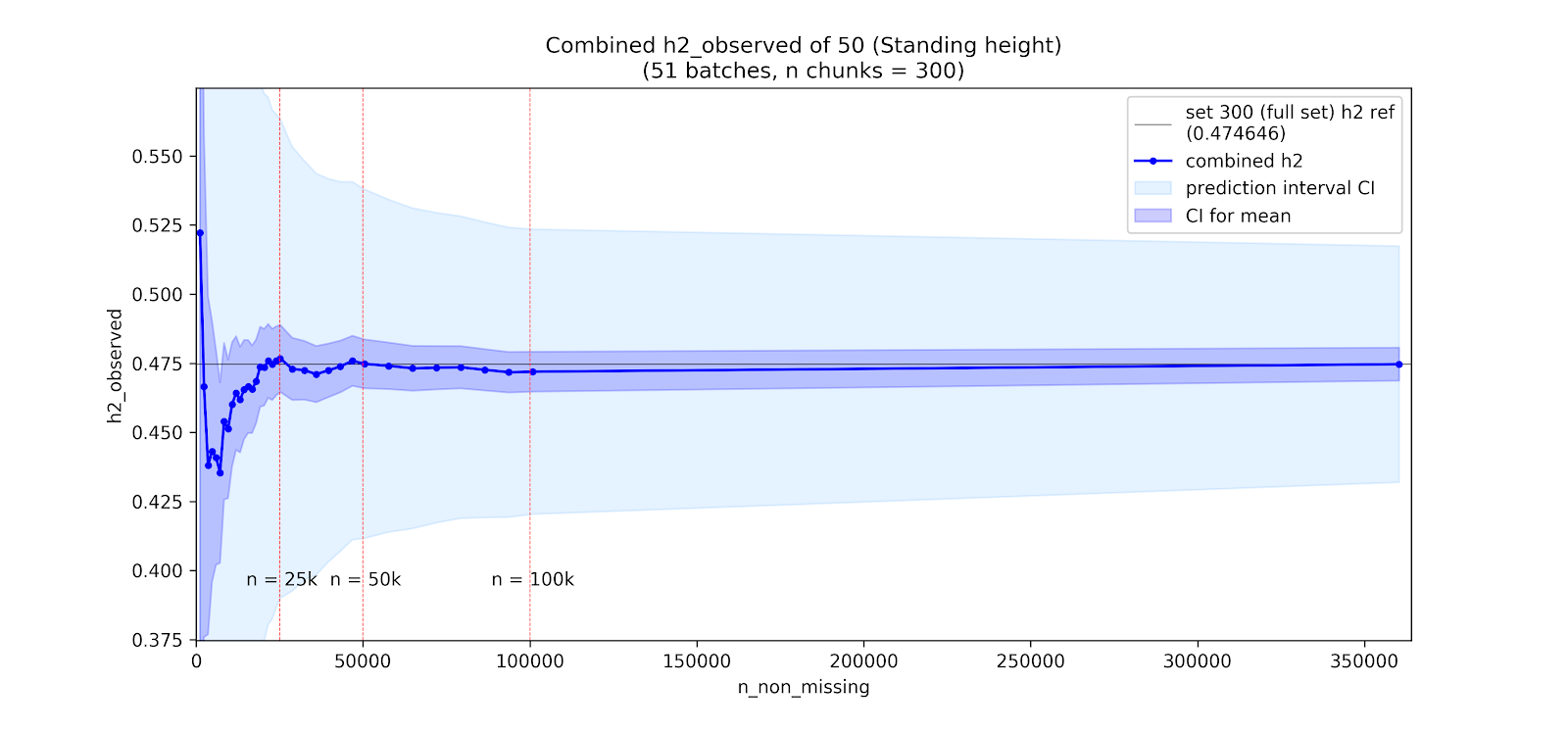
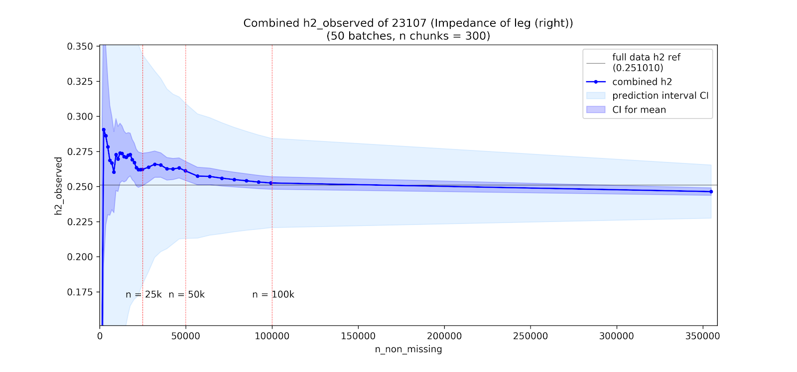
Note: Above are two specific examples among a broader set of ongoing analyses. Plots by Nikolas Baya.
Takeaway: There are signs of attenutation of the LDSR \(h^2_g\) estimate at low \(N\) in height, but leg impedence shows no such attentuation, and instead may have an upward bias. In both cases, estimates are clearly unstable at low \(N\).
Conclusion: These results are preliminary, and appear fairly unstable across phenotypes, but suggest that attenuation may occur irregularly across phenotypes and than in some instances there may be upward bias rather than downward attenuation at low sample sizes.
Question 3: Attentuation a function of stratification?
The downsampling experiments, while inconclusive, do suggest instability of the LSDR \(h^2_g\) at low \(N\), with variability possibly exceeding the SE estimates. Noteably, there were signs of attenuation at low \(N\) for height, a phenotype where the GWAS is likely affected by population stratification (intercept = \(1.313\), p = \(9.29\times 10^{-10}\), ratio = \(0.084\)), but not leg impedence where stratification is weaker (intercept = \(1.096\), p = \(5.53\times 10^{-5}\), ratio = \(0.053\)).
This leads us to evaluate whether the relationship between sample size and LDSR \(h^2_g\) varies as a function of stratification. We start by noting that the LDSR intercept is expected to estimate \(1+Na\) where \(N\) is sample size and \(a\) is an index of population stratification or other counfounding that is, under a simple stratification model, proportional to \(F_{st}\). It follows that \(a=(intercept-1)/N\) should give an estimate of stratification that is invariant to sample size.
On that basis, we look at LDSR \(h^2_g\) estimates as a function of \(N_{eff}\) split by deciles of \(a=(intercept-1)/N\).
Note: Plot restricted to \(N_{eff} < 200,000\) and \(|h^2_g|<.5\) for visibility.
From the above plot, we see a strong relationship between the trend in \(h^2_g\) at low sample sizes and \(a\) from the fitted intercept. These trends also continue in the sample sizes below \(N_{eff}=4500\) excluded above. Specifically, phenotypes at low \(N_{eff}\) with higher fitted intercepts (e.g. deciles 8-10) tend to have lower \(h^2_g\) estimates (to the point of the average estimate being negative), while phenotypes with lower fitted estimates (including \(a < 0\), which corresponds to intercepts below 1) have higher \(h^2_g\) estimates. Phenotypes with nearly null intercepts (deciles 3-4, \(a \approx 0\), intercept \(\approx 1\)) show no directional bias on average.
It’s worth noting that the trends conditional on estimated \(a\) are likely to reflect both:
- Effects of true stratification/confounding in the GWAS, such that the true value of \(a\) is non-zero
- Negative correlation of intercept and slope estimate from the LDSR regression when there’s insufficient power to differentiate signal from noise
- Unstable trends for the top/bottom decile due to limited phenotypes with low intercept alphas at high sample size, and (to a lesser extent) with high intercepts at low sample size.
The stability of the \(h^2_g\) estimates may also be connected to the intercept \(a\) even at high sample sizes. E.g. this is evident if we focus on the top 5 deciles of \(a\) in effective sample sizes above 100,000.
Nevertheless, to the extent the fitted \(a\) estimates don’t appear centered at zero (e.g. zero is covered by decile 3, mean \(a = 7.05\times 10^{-8}\), standard deviation \(= 2.38\times 10^{-7}\)) it is likely the \(a\) values do reflect some non-zero amounts of confounding/stratification in at least some of the phenotypes. It is unclear however to what extent the directional biases in \(h^2_g\) conditional on \(a\) reflect effects from the true value of \(a\) versus correlated sampling noise in the intercept and slope estimates.
The relationship to \(a\) may also explain why the attenuation at low \(N_{eff}\) is weaker in the Round 2 results than in Round 1. The Round 2 GWAS increased the number of PCA covariates and used PCs computed within the GWAS sample (i.e. within european ancestry individuals) rather than the PCs from the full UKB data (i.e. with all ancestries). As a result, stratification may be better controlled within the Round 2 results, thus any dependence of the \(h^2_g\) results on \(a\) at low \(N_{eff}\) will have a weaker marginal effect than in Round 1 due to reduced true values of \(a\).
Takeaway: In either case, it is clear from the first figure above that there is strong dependence between \(h^2_g\) and \(a\) at low \(N_{eff}\), with convergence to more stable \(h^2_g\) estimates regardless of \(a\) as \(N_{eff}\) increase (subject to the instability from sparse representation of the \(a\) decile or increased SEs of the \(h^2_g\) estimate).
Conclusion
From the plot of \(h^2_g\) by \(a\) decile, it appears LDSR \(h^2_g\) estimates converge to stabilty in the \(N_{eff}=20,000-40,000\) range. This is broadly consistent with the downsampling experiments above, though in some instances those show evidence of slightly slower convergence. Based on the above, we therefore denote our confidence in the LDSR \(h^2_g\) results as follows:
- \(N_{eff} < 4500\): No confidence (see minimum sample size requirements)
- \(4500 \leq N_{eff} < 20,000\): Low confidence
- \(20,000 \leq N_{eff} < 40,000\): Medium confidence
- \(N_{eff} \geq 40,000\): High confidence
[NB: Of the criteria in this LDSR analysis, this choice is probably the least stable. The downsampling experiments remain unclear about the nature of biases at low \(N_{eff}\), suggesting effects beyond what might be anticipated based on the full-sample estimate of \(a\). As a result, thoughts about best practices for interpreting \(h^2_g\) estimates in this intermediate range of \(N_{eff}\) are still very much subject to change.]
Unusually large standard errors
In assessing the minimum necessary sample size above, we noted the relationship between sample size and the SE of the \(h^2_g\) estimate. Although we focused on the average SE by sample size, it may also be observed that there are some clear outliers with larger SEs than would be anticipated based on their sample size.
We focus here on phenotypes that are at least medium confidence based on \(N_{eff}\).
The clearest outlier here is red hair color (from UKB code 1747). In addition to the disproportionately large SE on the \(h^2_g\) estimate for this phenotype, it also has a remarkably low intercept estimate which is also unstable (intercept = 0.619, SE = 0.387). A similar pattern is observed for the next two outliers, measures of bilirubin from the biomarker data (codes 30660 and 30840). Note that an intercept \(<1\) is unexpected under the LDSR model, where variants tagging no signal (LD score of 0) should have a null expectation of 1 (for the 1 df \(\chi^2\) statistic).
Looking at the manhattan plot for the red hair phenotype, it becomes clear that the genetic signal is dominated by two loci. The manhattan plots for bilirubin are similarly sparse with even stronger top loci (not shown).
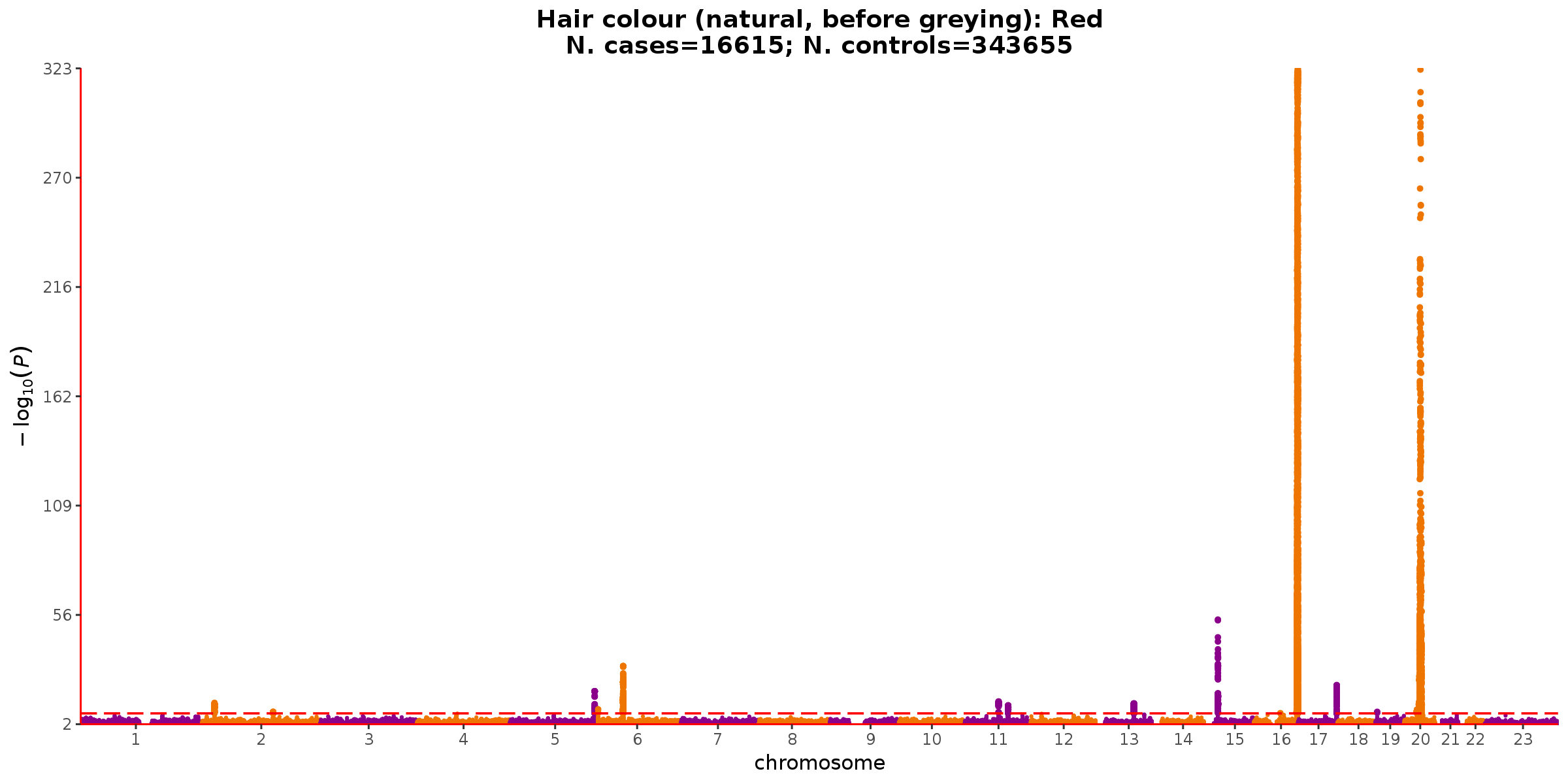
Note: y-axis truncated for MC1R locus on chromosome 16.
LDSR is derived assuming a broadly polygenic architecture for each trait. Although sparser polygenicity doesn’t fully invalidate the LDSR model (under a moments-based framework), it has previously been observed that LDSR is increasingly unstable for sparse architectures.
Although we hope that the reported SEs will accurately capture the instability of estimates for these phenotypes with sparse architectures, we may have lower confidence in these results. We may be particularly concerned about phenotypes where the SE is large and coupled with a low estimated intercept, which could in turn lead to over-estimation of \(h^2_g\).
Using the same loess fit as above to predict the expected SE based on \(N_{eff}\), we evaluate the ratio between the observed and expected SE along with the fitted intercept.
The top outliers are observed for pigmentation-related traits, which have architectures similar to red hair as illustrated above, and other biomarkers like bilirubin. Following the biomarkers, the next set of phenotypes with larger-than-expected SEs are haematology measures, such as thrombocyte volume (UKB code 30100).
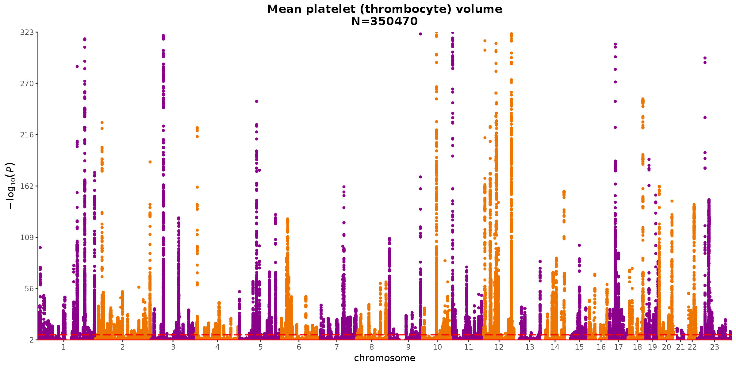
Takeaway: Thrombocyte volume also has loci of very strong effect, but in the context of a more polygenic architecture.
Although the unexpectedly large SEs for phenotypes like thrombocyte volume are still worrisome, they are less concerning than the stronger outliers for pigmentation-related traits and biomarkers like bilirubin whose GWAS signals are driven by only a handful of loci.
Conclusion
We mark reduced confidence in phenotypes with unexpectedly large SEs as follows:
- Low confidence: All hair color levels (UKB code 1747), plus other items with Observed/Expected SE ratios > 12 and intercepts < 1.1
- Medium confidence: All other items with Observed/Expected SE ratios > 6
All affected measures are pigmentation-related or biomarker or haemotology measures. [NB: Height (UKB code 50) is just barely under the 6x ratio of observed vs. expected SE. It’s a borderline decision. We choose to give it some leeway given the general trend that higher \(h^2_g\) also has higher SE and height has very strong \(h^2_g\).]
Sex-biased phenotypes
We noted when selecting primary results for each phenotype that although we were designating the both-sex analysis as the primary analysis where possible that we would revisit the question of results for phenotypes with a strong sex bias. We revisit that question here.
We first look at the sex balance of phenotypes using a both_sexes GWAS that passed the minimum sample size filters and have high confidence after the previous checks in this section.
Takeaway: Sample sizes are nicely balanced between sexes. The small tail of items with >60% female samples primarily consists of depression-related questions.
As before, we can similarly check the balance among cases and among controls for binary phenotypes.
Although these phenotypes are mostly balanced, there is a clear remaining tail of phenotypes with strong sex bias among cases.
We don’t have particularly strong reasons to be concerned about LDSR results for phenotypes with strong sex differences. Noteably the GWAS is already conditioned on sex as a covariate (as well as \(Sex \times Age\) interactions). On the other hand, we may have some concerns over whether the phenotype has the same meaning in both sexes or whether there are for example differential ascertainment biases affecting each sex in the GWAS sample. In both cases, this concern can be summarized as a worry over the potential for \(G \times Sex\) interactions (either in the population or as an artifact within sample). On that basis, we choose to flag phenotypes with strong sex differences in sample size as somewhat lower confidence.
Conclusion
We denote as “medium” confidence 15 phenotypes where >75% of cases are from a single sex.
[For reference, phenotypes narrowly avoiding the 3:1 threshold for reduced confidence here include: use of soy milk, taking vitamin D supplements, attending adult education classes, having gallstones, and additional headache and heart heath phenotypes.]
We only flag these phenotypes as “medium” confidence (as opposed to “low”) since this is an arbitrary threshold and is only being considered out of an abundance of caution. We would also flag phenotypes with >75% of total sample size or >75% of controls from a single sex, but no such phenotypes are present here. An additional 25 phenotypes that would meet these criteria for sex-biased prevalence are already marked as medium confidence due to limited sample size.
Ordinal coding issues
In reviewing the phenotypes for this GWAS release, it was noted that the automated phenotype processing with PHESANT used for the GWAS yielded a small number of phenotypes with poor/uninterpretable encodings of UKB participant answers. Specifically, the issue is variables identified as ordinal by PHESANT where the labels for the ordinal levels are non-sequential numeric values and/or do not reflect that natural numeric ordering/spacing of the available response categories. For most of the identified cases this would be fine if the ordinal phenotypes were being analyzed with e.g. ordinal logistic regression as originally intended by PHESANT, but since the Neale Lab GWAS uses linear regression for all phenotypes the ordinal coding does impact the current GWAS results.
We focus here on two categories of phenotypes:
Ordinal phenotypes whose levels are not coded as sequential integers
Ordinal phenotypes whose integer coding does not reflect the scaling of quasi-numeric response categories
Non-sequential ordinal coding
A review of the PHESANT output for the phenotypes in the Neale lab GWAS finds 7 phenotypes with non-sequential codes. In other words, there are phenotypes that are marked as ordinal variables but don’t end up with values of [1,2,...,k] or [0,1,...,(k-1)] (where \(k\) is the number of response categories) in the post-PHESANT phenotypes for GWAS. The 7 identified phenotypes are:
| Pheno. | Description | Ordinal Levels |
|---|---|---|
| 4270 | Volume level set by participant (left) | [10, 20, 40, 70, 100] |
| 4277 | Volume level set by participant (right) | [10, 20, 40, 70, 100] |
| 4814 | Tinnitus severity/nuisance | [4, 11, 12, 13] |
| 100010 | Portion size | [5, 10, 15] |
| 100400 | Standard tea intake | [0, 1, 2, 3, 4, 5, 600] |
| 102290 | Dark chocolate intake | [0, 1, 2, 3, 4, 6] |
| 104920 | Time spent doing light physical activity | [0, 1, 13, 35, 57, 79, 912, 1200] |
We review each of these in turn.
4270 and 4277 report the volume percentage selected by the participant. Although this is marked as ordinal, the response coding reflects the numerical level of the percentages. This is not problematic.
4814 codes reported tinnitis severity. It appears PHESANT missed recoding this variable, instead keeping the original UKB encoding of
4: Not at all,11: Severely,12: Moderately, and13: Slightly. Is it evident that both the ordering and scaling of the codes is problematic.100010 reflects the raw UKB encoding for portion size of
5: smaller,10: average, or15: largerthan normal portion sizes. Although a[1,2,3]encoding might be more conventional here, no harm is done by this alternate coding.100400 codes the number of cups of tea consumed, with a code of
600reflecting a reponse of6+. Obviously this coding gives dramatically outsized weight to the6+response in an unintended way, giving numeric weight to a placeholder value used by UKB to distinguish the6+response from a simple6. Using this value for GWAS is problematic.102290 codes chocolate intake, and correctly recodes/reorders from the placeholder values reported by UKB for the number of chocolate bars consumed:
444: quarterbecomes 1,555: halfbecomes 2,1: 1becomes 3,2: 2becomes 4,3: 3becomes 5,4: 4: becomes 6, and500: 5+becomes 7, with a default value of 0 added for people who took the corresponding diet questionanaire but didn’t report any chocolate intake. The non-sequential values occur because the the response categories for3and5+are dropped for having too few respondants. Dropping these levels may make sense for an ordinal regression, but is suboptimal for our linear regression. Giving thequarterandhalfresponse levels integer coding may also distort the phenotypic scaling in a linear regression. Thus in sum, the non-sequential codes are understandable but the encoding may still have issues; we return to this potentially error mode in the next section.104920 also appears to have missed recoding of the ordinal levels by PHESANT. The reported values conflate a range of hours spent on the activity (
0: None,1: Under 1 hour,13: 1-3 hours,35: 3-5 hours,57: 5-7 hours,79: 7-9 hours,912: 9-12 hours, and1200: 12+ hours). Like the tea intake item, these are clearly placeholders and not well-suited to GWAS. The clearly nonlinear relationship between these codes and the underlying number of hours being reported is likely problematic.
Takeaway: Phenotypes 4814, 100400, and 104920 are clearly problematic, phenotypes 4270, 4277, and 100010 are fine with their current codings, and phenotype 104920 is concerning but not severely broken. The next section considers additional phenotypes like 104920 with potentially nonlinear encodings.
Quasi-numeric ordinal phenotypes
As is evident in the ordinal phenotypes considered above, many of the ordinal phenotypes in UK Biobank reflect response options with some degree of numeric meaning. This is evident in the case of the diet items above, where even when converted to ordinal codings as intended by PHESANT (i.e. 102290) the result is fractional values getting treated as integers and thus a nonlinearity of the numeric treatment of the phenotype.
We therefore review the codings for all 264 ordinal variables to identify phenotypes whose codings potentially reflect nonlinear codings of implied numeric values in the response categories. Three examples of phenotype codes with this kind of potential issue are shown below:
Ever taken cannabis
| coding | meaning |
|---|---|
| 0 | No |
| 1 | Yes, 1-2 times |
| 2 | Yes, 3-10 times |
| 3 | Yes, 11-100 times |
| 4 | Yes, more than 100 times |
Dark chocolate intake
| coding | meaning |
|---|---|
| 1 | quarter |
| 2 | half |
| 3 | 1 |
| 4 | 2 |
| 5 | 3 |
| 6 | 4 |
| 7 | 5+ |
Duration of worst depression
| coding | meaning |
|---|---|
| 1 | Less than a month |
| 2 | Between one and three months |
| 3 | Over three months, but less than six months |
| 4 | Over six months, but less than 12 months |
| 5 | One to two years |
| 6 | Over two years |
Codes are shown after the recoding done by PHESANT. The cannabis item is especially illustrative since it shows the strongly nonlinearity potentially present in the ordinal codings while simultaneously showing a scenario where that nonlinearity may be desirable (e.g. focusing on comparison of use ever vs. occassionally vs. frequently).
After review, we identify a total of 30 response codings covering 80 phenotypes that appear at risk for this kind of nonlinear encoding of quasi-numeric response categories. A full list of the identified codings is available here. Because the ordinal encodings of these items may bias the GWAS results compared to a GWAS of the implied numeric quantity, we designate the \(h^2_g\) results for these ordinal phenotypes as “medium” confidence to reflect the impact on interpretability.
Note the chosen list of codings is intentionally broad, and thus this reduction of confidence is likely conservative. In many cases, the coding may be close enough to linear and/or may reflect intentional choices of a scale most informative for the phenotype (e.g. the cannabis coding above), and thus the reduced confidence is unnecessary. Nevertheless, we err on the side of caution, especially since we expect the “medium” confidence results to still be included for most uses of these \(h^2_g\) results, and thus use this opportunity to flag the affected ordinal phenotypes are deserving additional attention with regards to interpretation.
Conclusion
UKB phenotypes 4814, 100400, and 104920 are marked as “low” confidence due to clear problems with the numeric values of their non-sequenital coding of ordinal response categories.
A set of 241 ordinal phenotypes whose coded response levels may not fully reflect the numeric scaling of the items response categories are designated as “medium” confidence to highlight that additional follow-up may be required for interpreting their GWAS and \(h^2_g\) results.
Summary of confidence ratings
In sum, the above process leaves us with:
| Confidence | Count | Description |
|---|---|---|
| NA | 7507 | not the primary analysis (sex-specific subset, un-normalized, redundant) |
| None | 2298 | \(N_{eff} < 4500\) |
| Low | 703 | \(N_{eff} < 20000\), or \(SE > 12\times\) expected with low intercept, or bad ordinal coding |
| Medium | 372 | \(N_{eff} = 20000-40000\), or \(SE > 6\times\) expected, or >3:1 sex bias, or nonlinear ordinal coding of numeric values |
| High | 805 | remaining phenotypes |
We then consider the statistical significance of the \(h^2_g\) results where we have at least some confidence in the LDSR estimate.